Visualizing IDyOM outputs

This tutorial will cover some useful plotting in py2lispIDyOM. For an overview of the py2lispIDyOM functionality, see the README. In the current version, only limited basic plots are available.

In this tutorial, We will continue the sample example as in the 1_running_IDyOM_tutorial.ipynb, and plot some IDyOM outputs from that experiment, where the log folder is experiment_history/21-05-22_17.05.05/

Current version of py2lispIDyOM has the following types of basic plots:

1. simple_plot

2. selected_surprisal_entropy

3. all_surprisal

4. all_entropy

5. pianoroll_pitch_prediction_groundtruth

6. pianoroll_groundtruth_overall_surprisal

# import BasicPlot from viz module

import py2lispIDyOM as py2lispIDyOM
from py2lispIDyOM.viz import BasicPlot

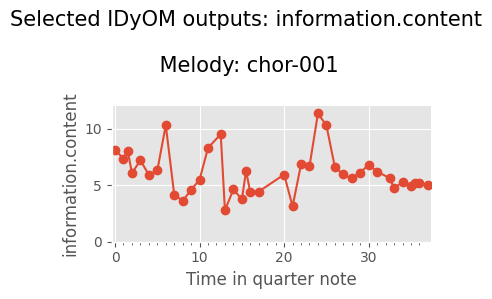
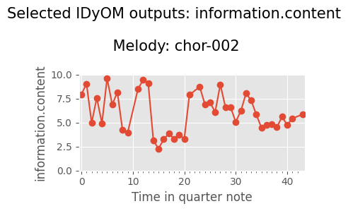
Simple Plot

BasicPlot.simple_plot

Generate a simple line plot with time (in quarter note) on the x-axis, and selected IDyOM output on the y-axis.

In the following example, we will:

- plot the `information.content` of the melodies named '"chor-001"', and '"chor-002"',
- save and show the figs here,
- use ggplot style and show grid.

Note that you can modify the figsize, dpi and other params as you like.

# specify experiment folder
my_exp = 'experiment_history/21-05-22_17.05.05/'

# specify plotting params
BasicPlot.simple_plot(selected_idyom_output= 'information.content',
                    experiment_folder_path=my_exp,
                    melody_names = ['"chor-001"', '"chor-002"'],
                    savefig = True,
                    showfig = True,
                    fig_format = 'png',
                    dpi = 100,
                    figsize = (4, 3),
                    grid = True,
                    ggplot = True)

simple_plot_information.content

Plots saved in experiment_history/21-05-22_17.05.05/plots/simple_plot_information.content/

Plots saved in experiment_history/21-05-22_17.05.05/plots/simple_plot_information.content/

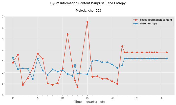
Selected surprisal and entropy

BasicPlot.selected_surprisal_entropy

Generate a figure that shows the selected entropy and information content.

In the following example, we will:

- plot the `onset.information.content` and `onset.entropy` of the melodies named '"chor-003"'
- save and show the figs here,
- use ggplot style and show grid.

# specify experiment folder
my_exp = 'experiment_history/21-05-22_17.05.05/'

# specify plotting params
BasicPlot.selected_surprisal_entropy(experiment_folder_path=my_exp,
                                    ic_source = 'onset.information.content',
                                    entropy_source = 'onset.entropy',
                                    melody_names = ['"chor-003"'],
                                    savefig = True,
                                    showfig = True,
                                    fig_format = 'png',
                                    dpi = 200,
                                    figsize = (10, 6),
                                    grid = True,
                                    ggplot = True)

selected_surprisal_entropy

Plots saved in experiment_history/21-05-22_17.05.05/plots/selected_surprisal_entropy/

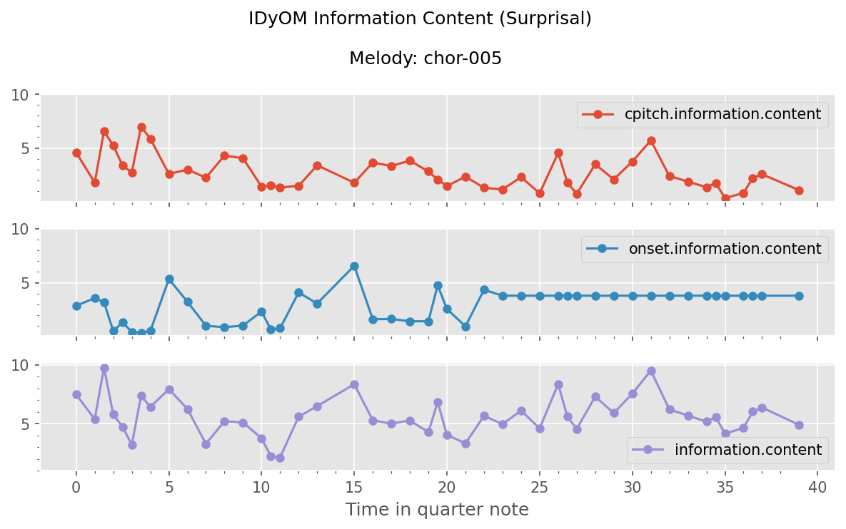
Plot all available surprisal outputs

BasicPlot.all_surprisal

Generate subplots of all available surprisal outputs.

In the following example, we will:

- plot the all available surprisal outputs of IDyOM of the melodies named '"chor-005"'
- save and show the figs here,
- use ggplot style and show grid.

# specify experiment folder
my_exp = 'experiment_history/21-05-22_17.05.05/'

# specify plotting params
BasicPlot.all_surprisal(experiment_folder_path=my_exp,
                        melody_names = ['"chor-005"'],
                        savefig = True,
                        showfig = True,
                        fig_format = 'png',
                        dpi = 150,
                        figsize = (8, 5),
                        grid = True,
                        ggplot = True)

surprisals_plots

Plots saved in experiment_history/21-05-22_17.05.05/plots/surprisals_plots/

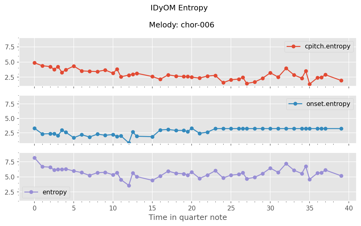
Plot all available entropy outputs

BasicPlot.all_entropy

Generate subplots of all available entropy outputs.

In the following example, we will:

- plot the all available surprisal outputs of IDyOM of the melodies named '"chor-006"'
- save and show the figs here,
- use ggplot style and show grid.

# specify experiment folder
my_exp = 'experiment_history/21-05-22_17.05.05/'

# specify plotting params
BasicPlot.all_entropy(experiment_folder_path=my_exp,
                        melody_names = ['"chor-006"'],
                        savefig = True,
                        showfig = True,
                        fig_format = 'png',
                        dpi = 150,
                        figsize = (8, 5),
                        grid = True,
                        ggplot = True)

entropy_plots

Plots saved in experiment_history/21-05-22_17.05.05/plots/entropy_plots/

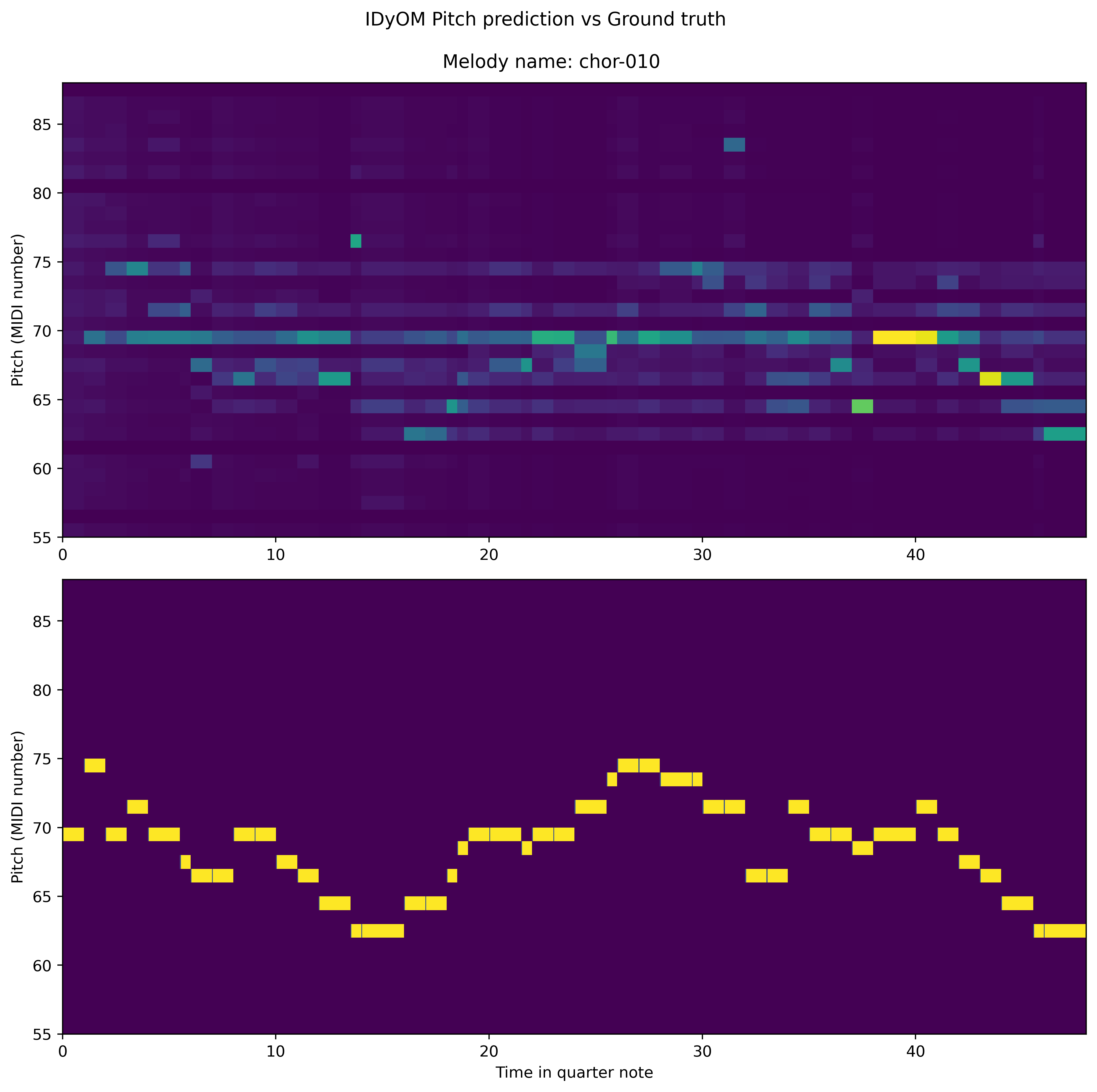
Plot piano roll of pitch prediction and ground truth

BasicPlot.pianoroll_pitch_prediction_groundtruth

Generate a pair of figures (the predicted pitch distribution and the ground truth) side by side. If users intend to plot figures for specific songs, they can do so by specifying either the melody names, or the starting/ending index in the melody list.

In the following example, we will:

- plot the melody named '"chor-010"'
- save the fig .

# specify experiment folder
my_exp = 'experiment_history/21-05-22_17.05.05/'

# specify plotting params
BasicPlot.pianoroll_pitch_prediction_groundtruth(experiment_folder_path=my_exp,
                                                melody_names = ['"chor-010"'],
                                                savefig = True,
                                                fig_format = 'png',
                                                dpi = 400)

pianoroll_pitch_prediction_groundtruth
Plots saved in experiment_history/21-05-22_17.05.05/plots/pianoroll_pitch_prediction_groundtruth/

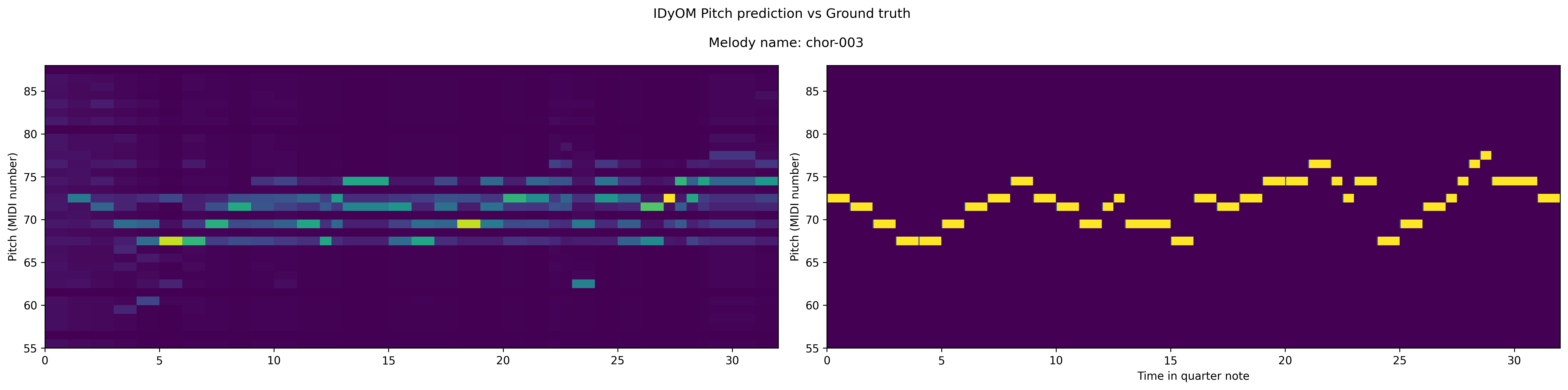
For some melodies that are relatively short and you may want to show the subplot side-by-side. You can do so by setting the nrows and ncols parameters

For example, in the following example, we will:

-  plot the melody named '"chor-003"'
- set the fig to show subplot side-by-side
- save and show the fig here.

# specify experiment folder
my_exp = 'experiment_history/21-05-22_17.05.05/'

# specify plotting params
BasicPlot.pianoroll_pitch_prediction_groundtruth(experiment_folder_path=my_exp,
                                                melody_names = ['"chor-003"'],
                                                savefig = True,
                                                showfig = True,
                                                fig_format = 'png',
                                                 figsize=(20,5),
                                                dpi = 300,
                                                nrows=1,
                                                ncols=2)

pianoroll_pitch_prediction_groundtruth

Plots saved in experiment_history/21-05-22_17.05.05/plots/pianoroll_pitch_prediction_groundtruth/

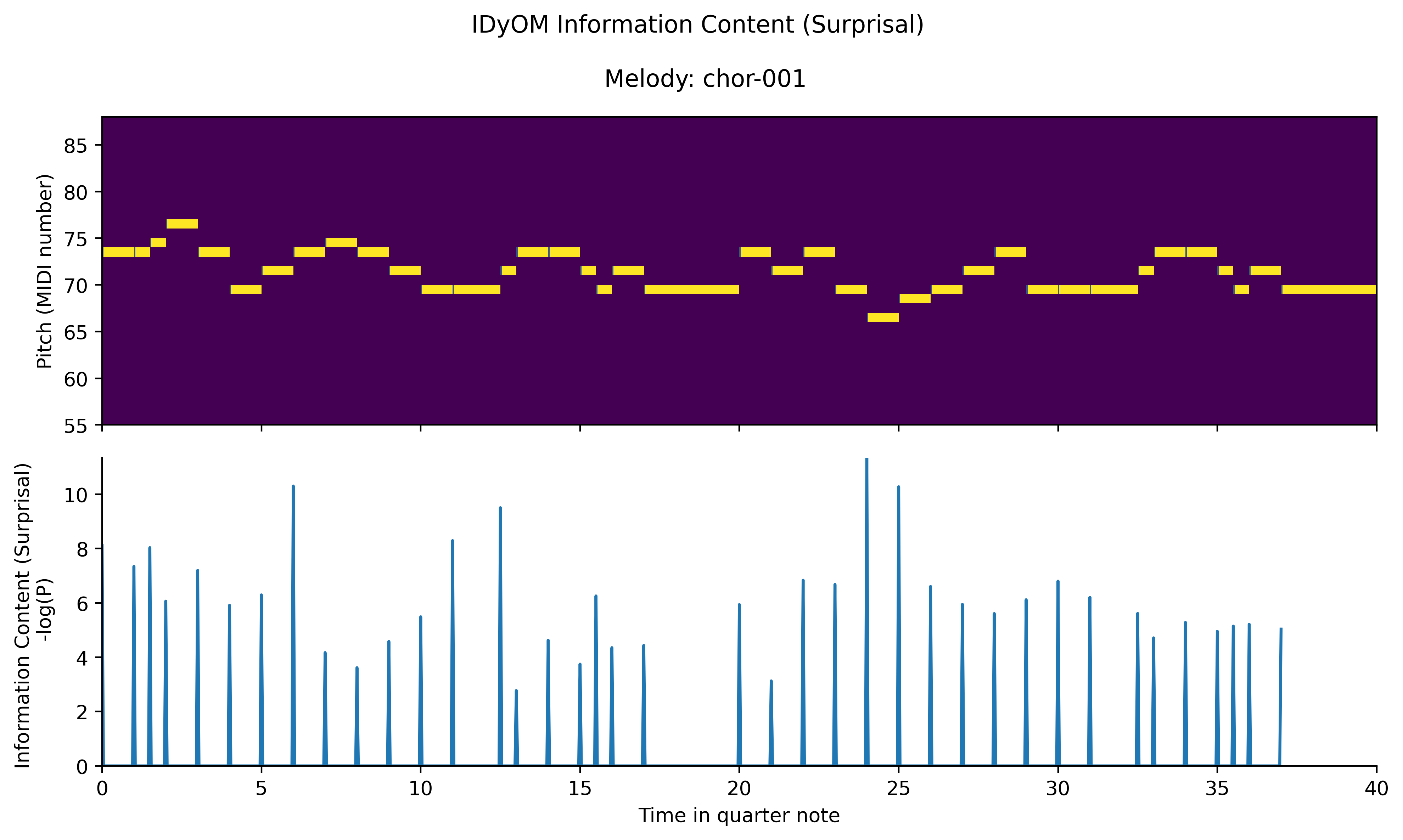
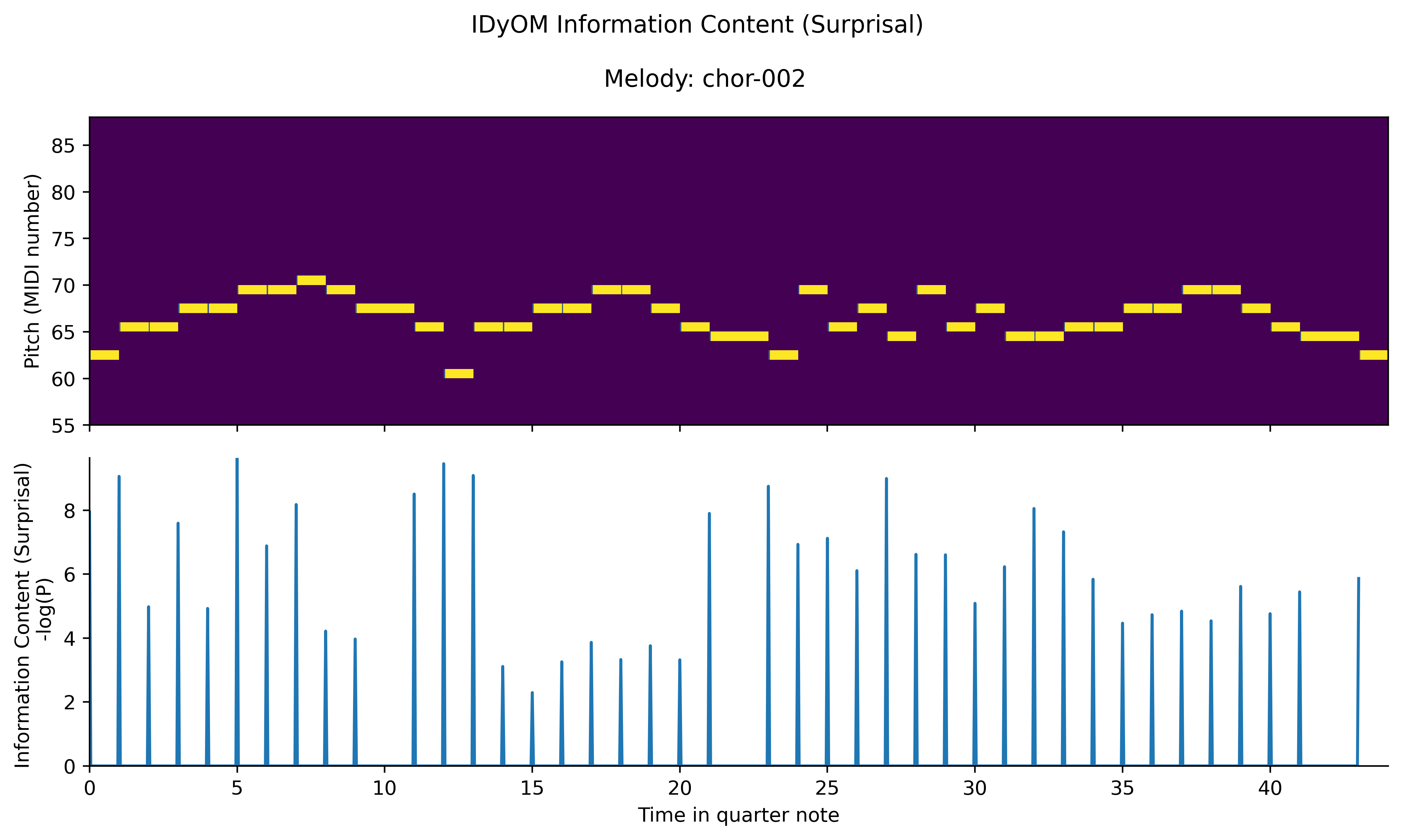
Plot piano roll of ground truth and overall surprisal (information content)

BasicPlot.pianoroll_groundtruth_overall_surprisal

Generate a pair of figures: ground truth piano roll on the top and the surprisal line plot on the bottom.

In the following example, we will:

- plot the first 2 melodies,
- save and show the fig here.

# specify experiment folder
my_exp = 'experiment_history/21-05-22_17.05.05/'

# specify plotting params
BasicPlot.pianoroll_groundtruth_overall_surprisal(experiment_folder_path=my_exp,
                                                starting_index=0,
                                                  ending_index=2,
                                                savefig = True,
                                                showfig = False,
                                                fig_format = 'png',
                                                dpi = 400)

pianoroll_groundtruth_surprisal
Plots saved in experiment_history/21-05-22_17.05.05/plots/pianoroll_groundtruth_surprisal/
Plots saved in experiment_history/21-05-22_17.05.05/plots/pianoroll_groundtruth_surprisal/